US Monetary Policy Rules | Leonardo Luksic

Background

Concepts & Research Design

The Taylor rule is a formula that describes how the Federal Reserve should adjust short-term interest rates in response to inflation deviating from a target (typically 2%) and unemployment deviating from its "natural" level. The structural form includes a smoothing parameter (ρ) that captures the Fed's tendency to adjust rates gradually rather than all at once. The equation estimated in this project is:

i_t = ρ · i_t−1 + (1 − ρ) · [r* + π_t + a_π(π_t − 2) + a_u(u_t − u_t^*)]

The Taylor principle is the key test of whether the Fed is doing enough to control inflation. It requires that when inflation rises by 1 percentage point, the Fed raises interest rates by more than 1 point (1 + a_π > 1), so that real (inflation-adjusted) borrowing costs actually increase. If 1 + a_π < 1, real rates fall during inflationary episodes, potentially allowing inflation to spiral.

Markov-switching models (Hamilton, 1989) identify distinct economic "regimes" from the data by estimating the probability of being in each state today given which state the economy was in yesterday. Unlike Gaussian Mixture Models, which cluster data points by similarity regardless of when they occurred, Markov-switching models account for temporal dependence, producing transition probabilities and expected durations for each regime. This matters because inflation regimes are persistent, not random.

CBO NAIRU (Non-Accelerating Inflation Rate of Unemployment) is the Congressional Budget Office's estimate of the time-varying natural rate of unemployment. It ranges from 4.3% to 6.2% over the sample period. Earlier studies used a fixed 5% benchmark, which overstates the unemployment gap during the 1970s and early 1980s when NAIRU was estimated at 5.8–6.2%.

Research Question

Does the Fed respond to inflation differently across regimes, and does the conventional finding of a structural break near 1980 survive more careful measurement?

The central finding is that the conventional story depends heavily on measurement choices. The 1980 structural break disappears when the unemployment gap is measured against time-varying NAIRU. The Taylor principle result differs depending on whether realized or expected inflation is used. And the apparent 12-month persistence of inflation is largely a statistical artifact of mixing two regimes with different average levels.

Analytical Approach

The analysis proceeds in four stages. First, regime identification using a 2-state Markov-switching model classifies each month into low or high inflation. Second, regime-conditional Taylor rules are estimated via nonlinear least squares with block-bootstrap HAC standard errors, using both realized and expected inflation. Third, structural break tests (sup-Wald, Chow) check whether the Volcker-era policy shift survives NAIRU-adjusted measurement. Fourth, forecasting experiments test whether regime awareness improves inflation prediction at horizons from 1 to 12 months.

Data

Sources & Variables

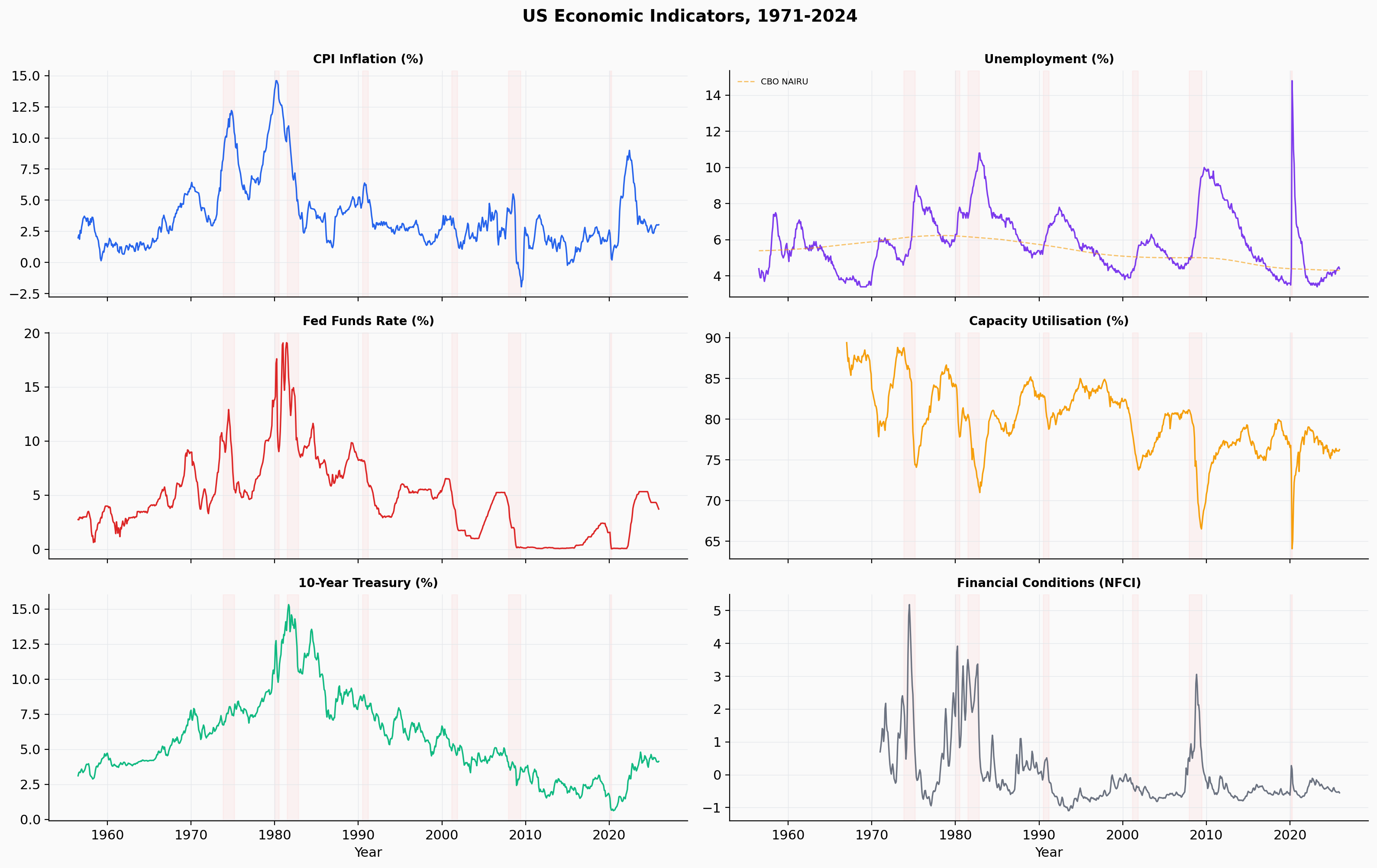
Eight monthly economic indicators from FRED, spanning July 1954 to December 2025. After merging and computing derived variables (inflation, gaps, lags, spreads), the working sample contains 833 monthly observations.

Monthly US economic indicators, 1954–2025. Recession periods shaded. The CBO NAIRU (dashed) varies from 4.3% to 6.2% over the sample.

Variable	FRED Series	Role
CPI	CPIAUCSL	Compute year-over-year inflation
Unemployment	UNRATE	Labour market slack
CBO NAIRU	NROU (quarterly, interpolated)	Time-varying natural rate for unemployment gap
Expected Inflation	MICH (from 1978; adaptive proxy before)	Forward-looking inflation measure
Fed Funds Rate	FEDFUNDS	Policy instrument (dependent variable)
Capacity Utilisation	TCU	Real-economy output measure
10-Year Treasury	GS10	Yield curve spread
Financial Conditions	NFCI (weekly, resampled monthly)	Financial stress indicator

833

Monthly Observations

71 yrs

1954–2025

NBER Recessions

Fed Chairs

Part I

Inflation Regimes

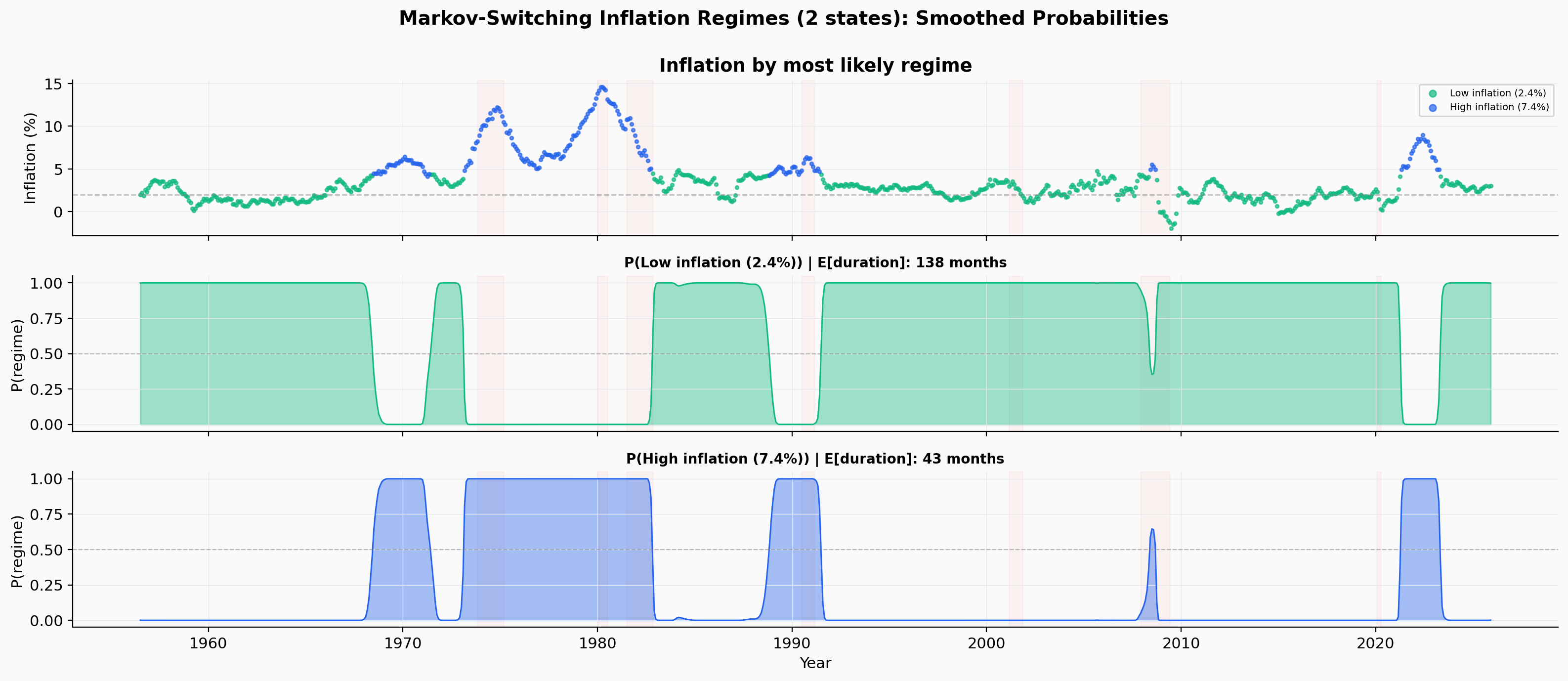
The US economy does not have one stable inflation rate. It alternates between distinct regimes with different typical inflation levels, different volatility, and different persistence. The 2-state Markov-switching model identifies a low-inflation state (average 2.4%, expected duration 11.5 years) and a high-inflation state (average 7.4%, expected duration 3.6 years).

Smoothed regime probabilities from the 2-state Markov-switching model. The high-inflation regime concentrates in the 1970s and early 1980s, with a brief reappearance during the post-COVID episode.

Regime	Mean π	Mean u	Mean FFR	Spread	E[Duration]	N
Low inflation	2.4%	5.8%	3.6%	+1.33 pp	11.5 yrs	622
High inflation	7.4%	6.0%	8.0%	−0.05 pp	3.6 yrs	211

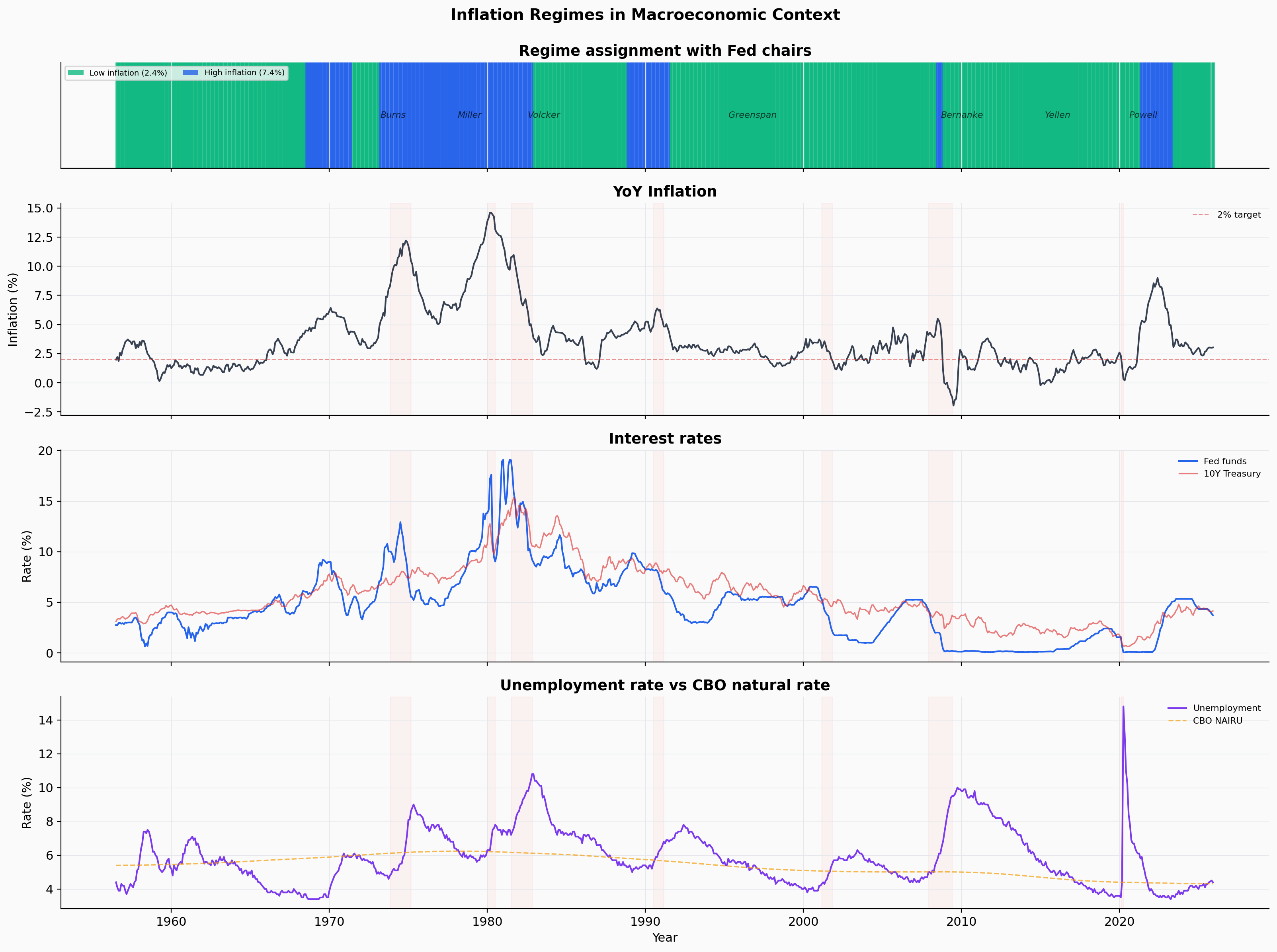
Inflation regimes overlaid on macroeconomic context. Chair tenures labelled. Bottom panel: unemployment against CBO NAIRU, which varies from 4.3% to 6.2% over the sample.

Monthly transition probabilities are high for both states: P(stay low) = 0.993 and P(stay high) = 0.977. The low-inflation regime lasts roughly three times as long on average, reflecting the difficulty of transitioning out of high inflation versus the relative stability of anchored expectations. BIC favours a 4-regime specification, but the 4-regime model has a near-singular covariance matrix (condition number 2.55 × 10¹⁸), making individual parameter estimates unreliable. The 2-regime model is retained as the primary specification.

Robustness: Pre-2020 Sample

Re-estimating on data ending at 2019:12 produces stable parameters: the low-inflation mean shifts from 2.4% to 2.3%, the high-inflation mean from 7.4% to 6.5%, and transition probabilities barely move. The regime structure is not driven by the post-2020 price dynamics.

Part II

Regime-Conditional Taylor Rules

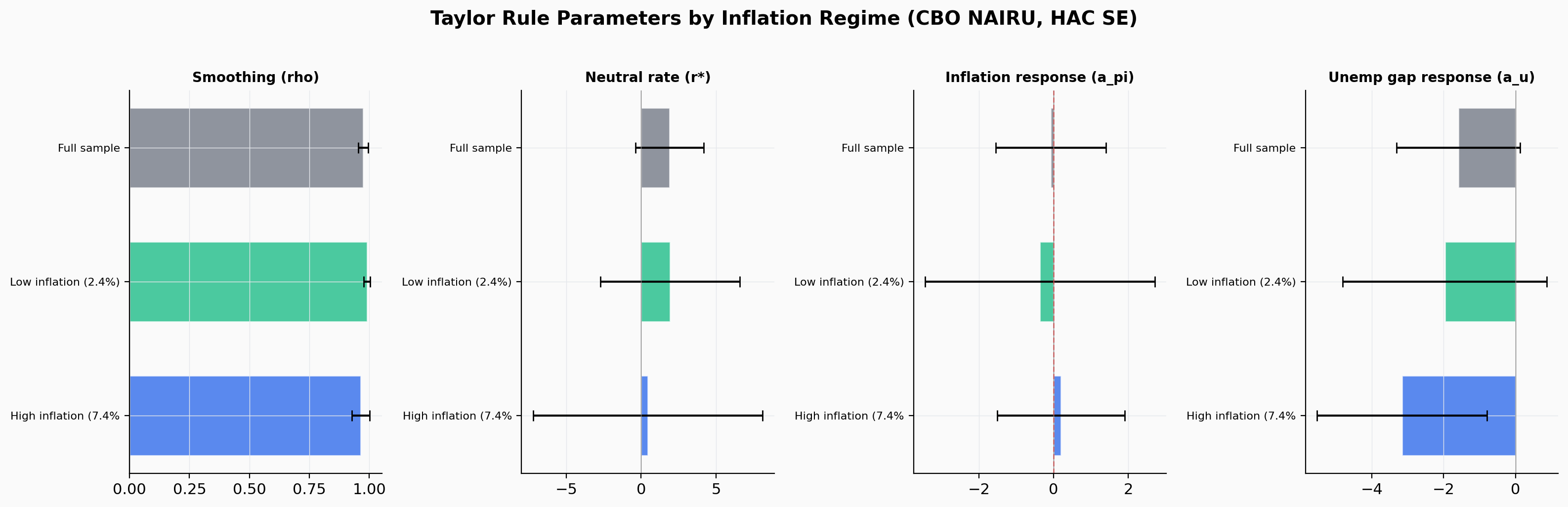
The structural Taylor rule is estimated via nonlinear least squares within each inflation regime, using CBO NAIRU for the unemployment gap. Standard errors are corrected for serial correlation using a block bootstrap (resampling year-long blocks of data 500 times). Both realized CPI inflation and expected inflation (Michigan Survey of Consumers) are tested.

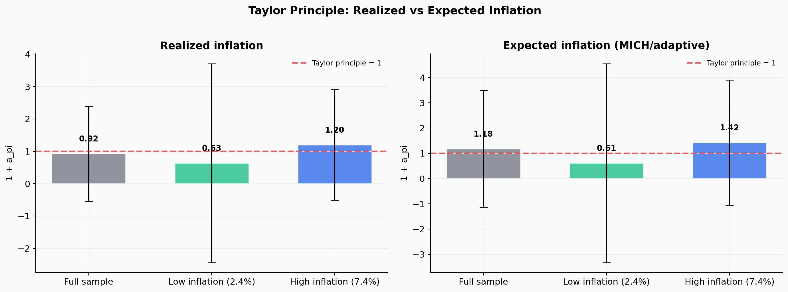
Structural Taylor rule parameters estimated within each inflation regime. Error bars show 95% HAC-bootstrapped confidence intervals, substantially wider than naive OLS standard errors.

Realized Inflation Specification

Sample	ρ	r*	a_π	a_u	1 + a_π	Taylor Principle
Full sample	0.974	1.90	−0.08	−1.59	0.92	Violated (point est.)
Low inflation	0.991	1.92	−0.37	−1.97	0.63	Violated
High inflation	0.964	0.45	0.20	−3.16	1.20	Weakly satisfied

Expected Inflation Specification

Using Michigan Survey of Consumers expected inflation (from 1978), with an adaptive expectations proxy (trailing 12-month mean of realized inflation) for earlier periods.

Sample	ρ	r*	a_π	a_u	1 + a_π	Taylor Principle
Full sample	0.979	1.77	0.18	−2.16	1.18	Weakly satisfied
Low inflation	0.992	1.83	−0.39	−2.30	0.61	Violated
High inflation	0.973	1.26	0.42	−4.34	1.42	Satisfied

The Taylor principle (1 + a_π) by regime under both specifications. The expected-inflation specification produces a clearer separation.

The difference between specifications is itself a finding: the Fed appears to have tracked expected rather than realized inflation, consistent with Boivin (2006). Using realized inflation understates the policy response because the Fed was reacting to its own forecasts, not to outcomes. With expected inflation, the high-inflation regime satisfies the Taylor principle at 1.42; with realized inflation, it does not clearly satisfy it in either regime.

Why Standard Errors Matter Here

Standard confidence intervals assume independent observations. Monthly economic data is not independent: this month's inflation is highly correlated with last month's. The block bootstrap (resampling year-long blocks 500 times) produces more honest uncertainty estimates. After correction, se(a_π) triples from 0.24 to 0.67, and the 95% CI on the Taylor principle spans [−0.39, 2.23], encompassing both violation and satisfaction. The point estimates are informative, but the uncertainty is real.

Prescription vs. Actual

Taylor Prescription vs. Actual Policy

If the Fed followed the estimated Taylor rule exactly, what interest rate would it prescribe at each point in time? The gap between this "prescribed" rate and the actual rate reveals when the Fed was tighter or looser than the rule implies. The rule is re-estimated at each month using only data available up to that point, so the prescription reflects real-time information.

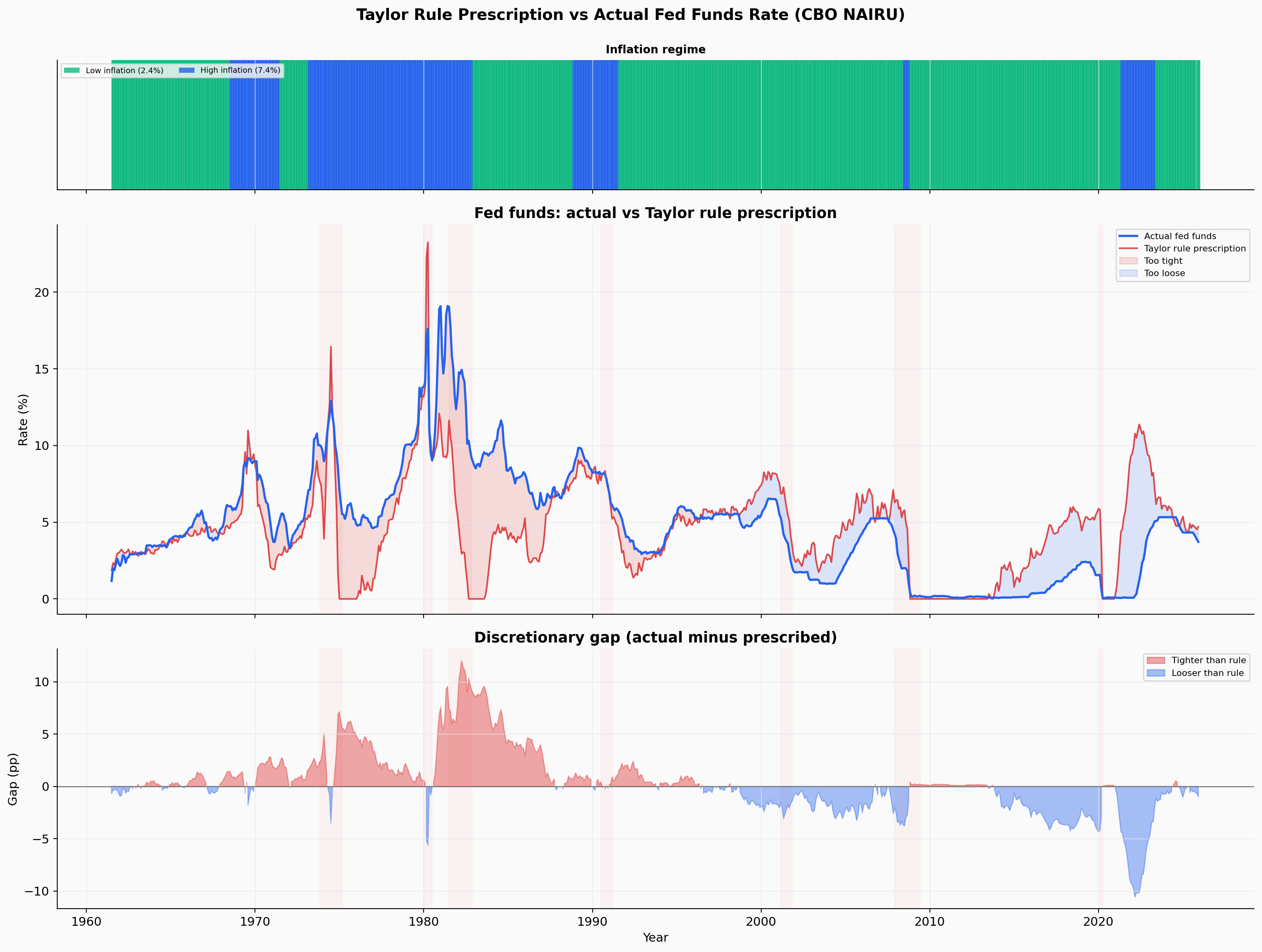
Expanding-window Taylor rule prescription (red) versus actual fed funds rate (blue). Bottom panel: discretionary gap, coloured by direction.

+0.31 pp

Mean Discretionary Gap

−0.07 pp

Gap in Low-Inflation Regime

+1.34 pp

Gap in High-Inflation Regime

With NAIRU-adjusted measurement, the average discretionary gap is near zero (+0.31 pp), in contrast to the large negative gap found with a fixed 5% benchmark. In the low-inflation regime, the Fed tracks the rule closely (−0.07 pp). In the high-inflation regime, the Fed was actually tighter than the rule would prescribe (+1.34 pp), reflecting the Volcker-era commitment to disinflation beyond what the estimated rule implied.

Part III

Structural Break Detection

A structural break is a point in time where the statistical relationship between variables permanently changes. Previous research (Clarida, Gali and Gertler, 2000) found a decisive break around 1980 when Volcker took over: the Fed supposedly started responding much more aggressively to inflation. The sup-Wald test checks every possible break date and identifies the most statistically significant one.

When the unemployment gap is measured against CBO's time-varying natural rate rather than a fixed 5%, no candidate break date exceeds the statistical significance threshold. The apparent break near August 1980 found in earlier work does not survive this more careful measurement.

Why the Break Disappears

CBO NAIRU varies from 4.3% to 6.2% over the sample. In the 1970s and early 1980s, NAIRU was estimated at 5.8–6.2%, well above 5%. Using a fixed 5% benchmark overstated the unemployment gap during this period, making the reaction function appear to respond differently before and after Volcker. When the gap is measured against the time-varying natural rate, some of what looked like a change in policy was actually a change in labour market structure.

The Chow test at the 1982–83 transition remains marginally significant (F = 2.94, p = 0.03), but the break is not dominant enough to survive the sup-Wald procedure. The Greenspan, Bernanke, Yellen, and Powell tenures remain statistically indistinguishable from each other.

Yield Curve

Recession Prediction & Regime Transitions

The "yield curve" refers to the gap between long-term and short-term interest rates. When long-term rates fall below short-term rates (an "inversion"), it has historically signalled an approaching recession. Two questions are tested: does this signal also predict inflation regime transitions, and how reliable is the recession signal when evaluated one episode at a time?

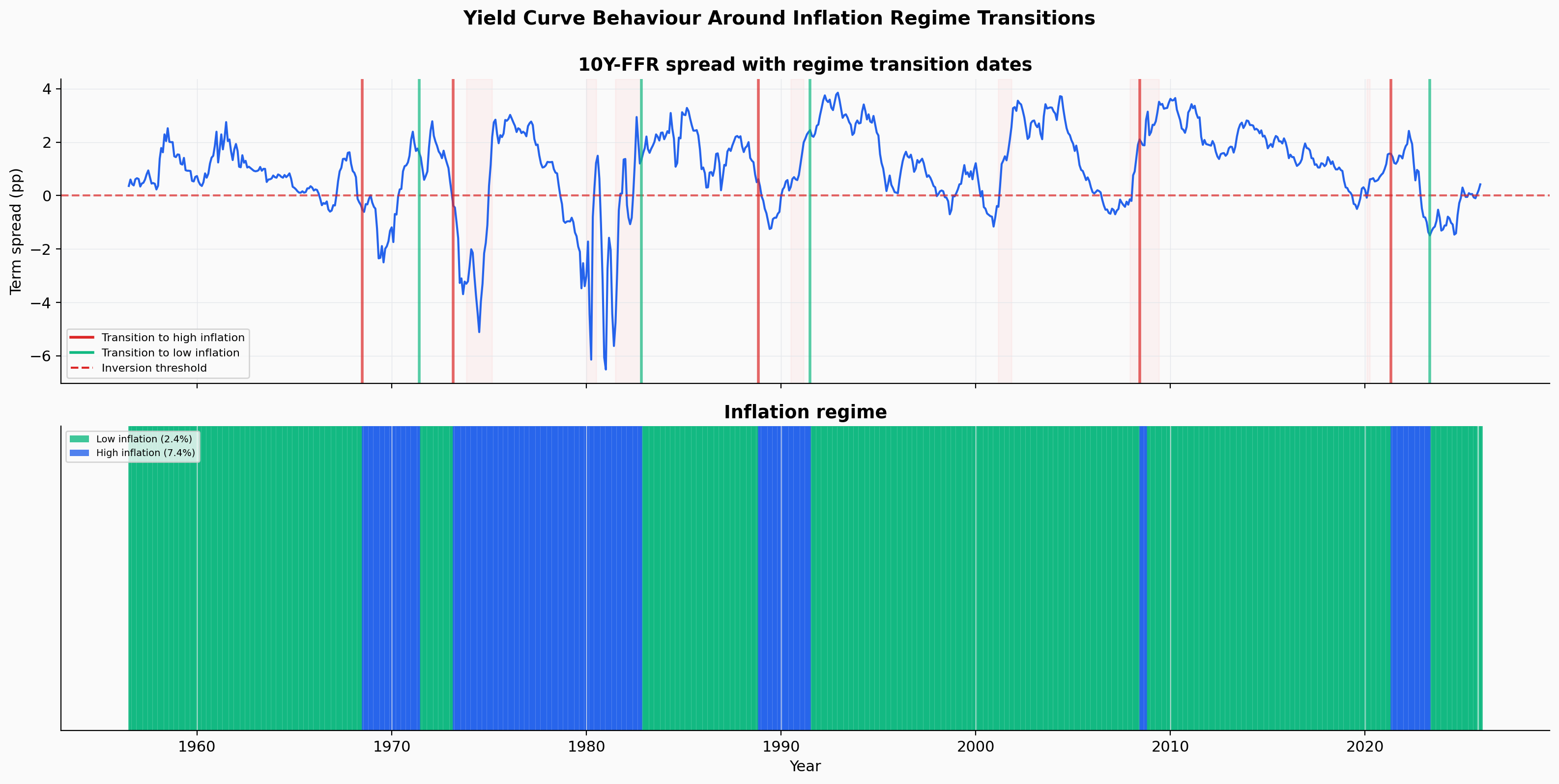
10Y-FFR spread with regime transition dates overlaid. Inversions precede some transitions but the relationship is not systematic.

Null Result: No Regime-Transition Signal

Logistic regression of "regime change within 12 months" on the term spread: coefficient = −0.009, p = 0.89. The bond market's recession-prediction ability operates through expectations of future rate cuts, a different channel from the supply shocks and expectation anchoring that drive inflation regime dynamics.

Recession Prediction Robustness

Standard tests train on early data and test on later data, which can be misleading if some recessions are easier to predict than others. Instead, leave-one-recession-out (LORO) cross-validation trains the model on six recessions and tests on the held-out episode, repeated for each of the seven recessions.

Recession	Full Model AUC	Spread-Only AUC
1973–74 Oil Crisis	0.939	1.000
1980 Volcker I	0.746	0.842
1981–82 Volcker II	1.000	0.838
1990–91	0.279	0.314
2001 Dot-com	0.750	0.750
2007–09 GFC	0.490	0.350
2020 COVID	1.000	0.995
Average LORO	0.743	0.727

The average LORO AUC (0.74) is substantially below the simple time-split estimate (0.78). Performance varies widely: the model fails on the mild 1990–91 recession (AUC 0.28) and the 2007–09 GFC (AUC 0.49), while COVID is trivially predictable from extreme preceding indicators. The yield curve is a useful but unreliable recession signal.

Part IV

Inflation Forecasting

Can knowing which inflation regime the economy is in help predict future inflation? Six forecasting approaches are compared at horizons from 1 to 12 months, using expanding cross-validation (train on all past data, test on the next period). R² measures forecast quality: positive means the model beats a naive guess of the historical average; negative means it does worse.

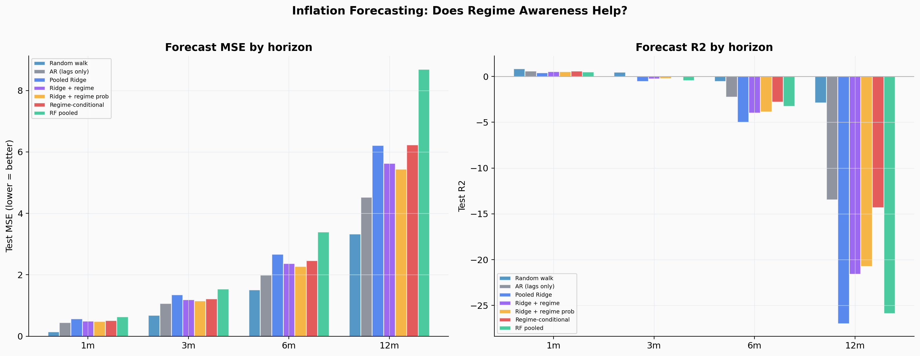
Forecast MSE and R² by horizon. All models produce positive R² at 1 month, but performance deteriorates rapidly; by 6 months, no model outperforms the historical mean.

Model	1m R²	3m R²	6m R²	12m R²
AR (lags only)	+0.62	+0.04	−2.23	−13.4
Pooled Ridge	+0.43	−0.53	−4.98	−27.0
Ridge + regime indicator	+0.54	−0.26	−3.99	−21.6
Ridge + regime probabilities	+0.55	−0.23	−3.84	−20.7
Regime-conditional	+0.61	+0.03	−2.78	−14.3
Random Forest	+0.51	−0.43	−3.25	−25.9

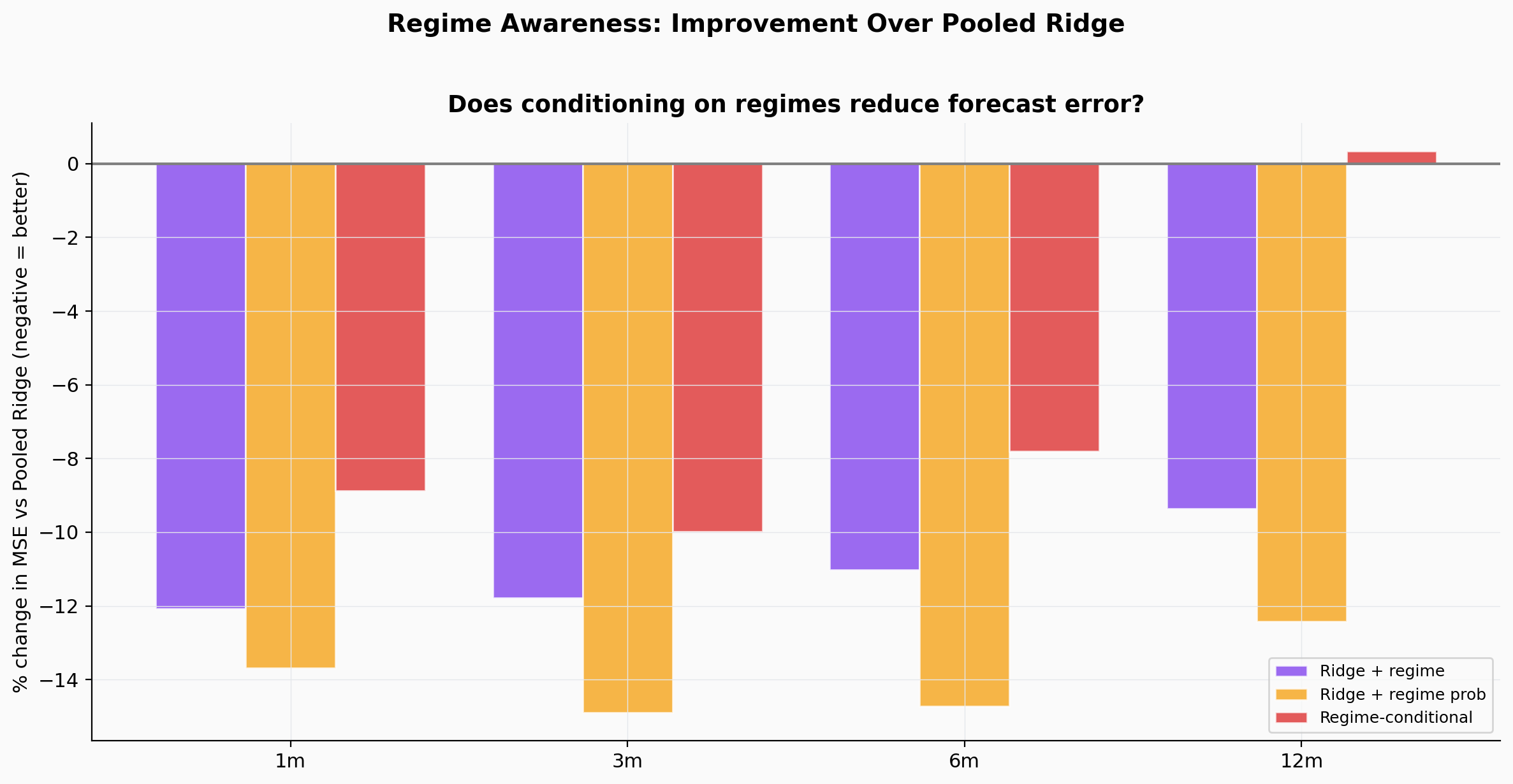
Percentage change in MSE from regime-aware models vs. the pooled Ridge baseline. Negative values indicate improvement.

At 1 month, the simple AR is hard to beat (R² = 0.62). The regime-conditional model comes close (0.61). At 3 months, only the AR and regime-conditional model produce positive R². By 6 months, all models are worse than the historical mean. Regime awareness identifies which distribution you are sampling from, but not where within that distribution the economy will be a year out.

Why 12-Month Forecasting Fails

Autocorrelation measures how much this month's inflation tells you about inflation N months from now. A value near 1 means strong predictability; near 0 means little signal remains.

Sample	AC(1)	AC(3)	AC(6)	AC(12)
Low-inflation regime (n=622)	0.950	0.792	0.598	0.283
High-inflation regime (n=211)	0.987	0.934	0.816	0.505
Full sample	0.990	0.955	0.893	0.731

This is an instance of Simpson's paradox. Full-sample autocorrelation at 12 months is 0.73, which makes inflation appear persistent and forecastable a year ahead. But this is mostly because the sample mixes periods of low inflation (averaging 2.4%) with periods of high inflation (averaging 7.4%). Within the low-inflation regime, AC(12) drops to 0.28. Roughly 40–60% of the apparent persistence comes from mixing the two distributions, not from inflation actually being predictable within either one.

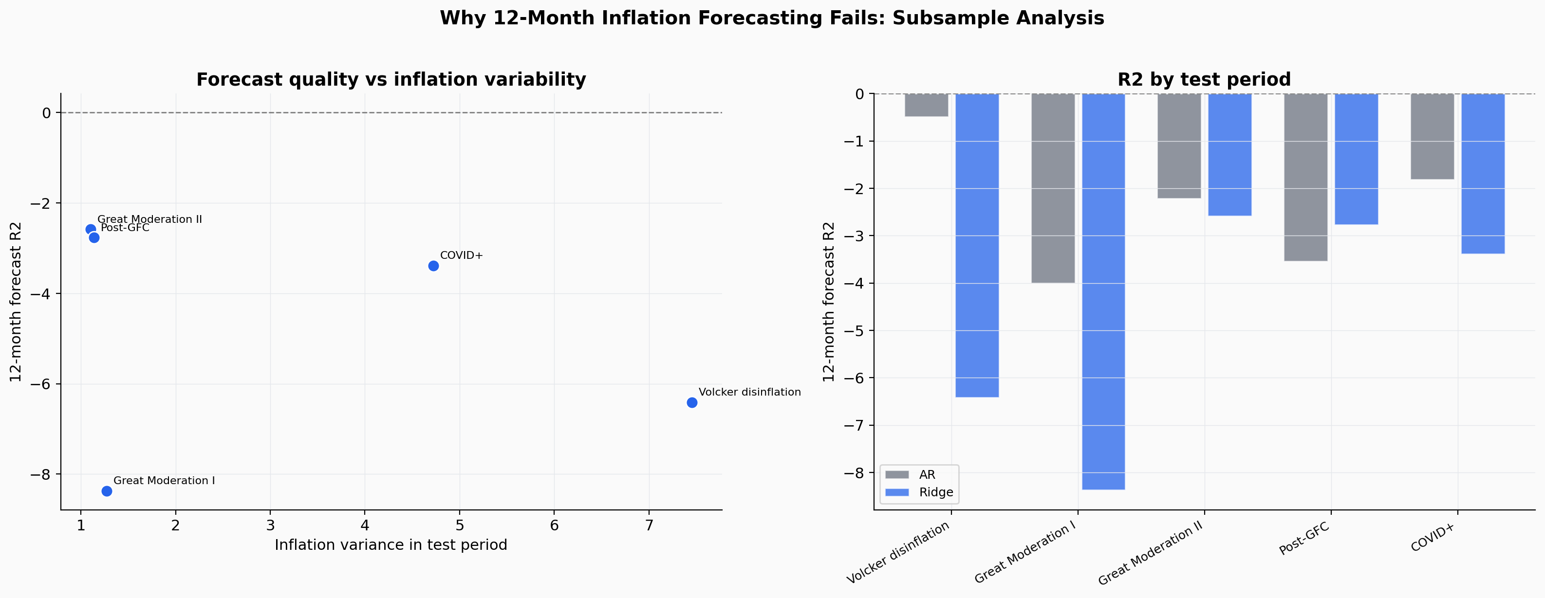
12-month forecast R² is negative across every historical subsample, regardless of model. The forecasting failure is structural.

Synthesis

Conclusions

The regime-switching, Taylor rule, structural break, and forecasting results point to four main findings about US monetary policy over the past seven decades.

Specification determines the Taylor principle result

With CBO NAIRU and expected inflation, the principle is satisfied in the high-inflation regime (1.42) but not the low-inflation regime (0.61). With realized inflation, it is not clearly satisfied anywhere. HAC standard errors are large enough that neither regime is statistically distinguishable from the threshold.

No structural breaks with time-varying NAIRU

The apparent structural break near 1980 disappears when the unemployment gap is measured against CBO NAIRU. Some of what looked like a change in policy behaviour was a change in labour market structure. The Chow test at 1982–83 remains marginally significant (p = 0.03), but the sup-Wald procedure does not detect a dominant break.

Inflation persistence is largely compositional

Inflation's apparent 12-month persistence is 40–60% a statistical artifact of mixing two regimes with different average levels. Within either regime, the forecasting signal decays rapidly. All models fail beyond 3 months in every subsample tested.

Simple models outperform complex ones

The 4-parameter structural Taylor rule recovers interpretable coefficients. The AR(12) is the strongest forecasting model at short horizons. The logistic regression with the term spread alone performs comparably to multivariate classifiers. With 833 observations spanning multiple structural regimes, complex models tend to overfit and deteriorate when conditions shift.

Limitations

Standard Errors

Even with block-bootstrap HAC correction, the standard errors on Taylor rule coefficients are large enough to make the core results statistically ambiguous. The very high smoothing parameter (ρ > 0.96) absorbs most variation, leaving little for other coefficients. This is a feature of the data, not a fixable estimation problem.

Expected Inflation Proxy

The Michigan Survey is available only from 1978. For the pre-1978 period, a trailing 12-month mean of realized inflation serves as an adaptive expectations proxy. This is a rough approximation that may not capture the Fed's actual information set during the Burns era.

Regime Model Stability

The Markov-switching model produces near-singular covariance matrices for some parameters. Regime assignments are reliable but standard errors on individual coefficients should be interpreted with caution. BIC prefers 4 regimes, but the 4-regime model has severe numerical instability.

Real-Time Data

All estimates use revised data. Real-time vintage data (what the Fed actually observed at each decision point) would provide a stricter test of the Taylor rule's descriptive accuracy. The break test uses the first-difference reaction function, not the structural NLS form.

Methodological Notes

Data Processing

8 monthly series from FRED (1954–2025). CBO NAIRU interpolated from quarterly to monthly. Michigan Survey from 1978; adaptive proxy (trailing 12-month CPI mean) for earlier periods. Derived variables: YoY inflation, unemployment gap (NAIRU-adjusted), term spread (10Y - FFR), capacity gap. 833 complete monthly observations.

Statistical Methods

Markov-switching: 2-state model (Hamilton 1989), EM algorithm. Taylor rule: nonlinear least squares, block-bootstrap HAC SE (500 draws, 12-month blocks). Break tests: Chow test, sup-Wald (Andrews 1993). Forecasting: expanding-window CV, 6 models (AR, pooled Ridge, Ridge + regime, regime-conditional, Random Forest), 4 horizons (1, 3, 6, 12 months). Recession prediction: logistic regression, LORO CV across 7 NBER recessions.

Authors: Leonardo Luksic, Krisha Chandnani, Ignacio Orueta

References: Hamilton (1989), Econometrica; Taylor (1993), Carnegie-Rochester Conference; Clarida, Gali & Gertler (2000), QJE; Andrews (1993), Econometrica; Bai & Perron (1998), Econometrica; Lubik & Schorfheide (2004), AER; Boivin (2006), JMCB; Stock & Watson (2007), JMCB.

Markov-Switching Nonlinear Least Squares Block Bootstrap HAC Sup-Wald Break Test Time Series CV FRED Data Python Statsmodels Scikit-learn